
Testing patterns of dispersion and codispersion of points is one of the most basic problems in point pattern analysis, but such tests (which are really intended for examining endogeneous spatial processes) can be easily confounded by dependency of the intensity function on underlying covariates. This is a huge problem in applied spatial statistics because most landscapes are highly heterogeneous and the inhomogeneity associated with such heterogeneity potentially invalidates statistical inferences (about clustering) based on popular summary functions, such as Ripley’s K.
In the last several decades, the development of inhomogenous versions of these summary functions has provided new opportunities to test hypotheses about dispersion and codispersion, and such functionality has become become readily accessible to spatial analysts via powerful open source packages in R such as ‘spatstat.’ The beauty of using a statistical programming languages such as R (rather than point and click GUIs) is that you can combine available functionality with custom scripts to conduct analyses that would otherwise be impossible.
In this blog post I am going to demonstrate such power using the codispersion of gopher tortoise and armadillo burrows as an example. Gopher tortoises and armadillos are both primary excavators of burrows (i.e., holes/tunnels in the ground) that they use as refuges. In the southeastern United States there is a lot of interest in how armadillos might be affecting gopher tortoises because, over the last 100 years, armadillos have expanded their range and now occur syntopically with gopher tortoises in many areas (where only gopher tortoises existed previously). These animals may be able to coexist because they have different diets, but armadillos are a major nest predator of gopher tortoises and there have been observations of agnostic interactions between the two species. Hence, one basic question involves whether the burrowing processes are independent against the alternatives that there might be repulsion or attraction of burrow types.
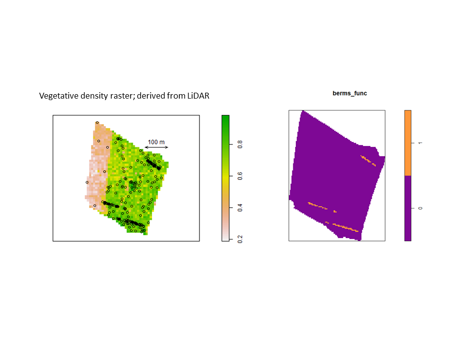
Nevertheless, the fact that one or both species often exhibit burrow patterns that show evidence of inhomogeneity prevents a simple test of independence (based on random displacement of the point patterns relative to one another). In this situation, your best option is to “Model and Monte Carlo”: model the inhomogeneity (using a multitype Poisson point-process model or by specifying an interaction between the covariates and the marks in an inhomogeneous Poisson point-process model) and then use the model to simulate appropriate random patterns and to estimate the intensity (for the purpose of correction with an inhomogeneous summary function). For example, numerous studies have asserted that armadillos prefer to burrow in areas with higher vegetative density and that they also prefer to burrow on sloped surfaces. Hence, technologies such as LiDAR can potentially be used to generate covariate surfaces that can be used as predictors in a point process model. For example, below (left) is a numeric covariate surface representing vegetative density (‘veg.cov.im2’). The other surface (right) is a factor-valued tessellation representing whether burrows are located inside or outside the areas of dirt berms (‘berms_func’).
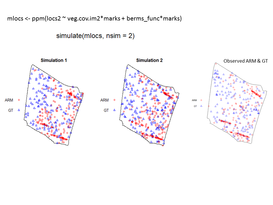
 To illustrate the utility of the Model and Monte Carlo approach, have a look at the two slides (below). In the first slide, the observed pattern (on the right side of the slide) is compared to two simulations based on complete spatial randomness and independence (CSRI). In this case, it would be inappropriate to use CSRI as a null model because we expect the armadillo burrows (red circles) to exhibit higher intensities on dirt berms and in areas with higher vegetative density (note that simulations based on CSRI do not look anything like the observed pattern). The second slide shows simulations based on an inhomogeneous Poisson point-process model with interactions specified between the marks and the two covariate surfaces (above) that seem to explain variation in the intensity of armadillo burrows.
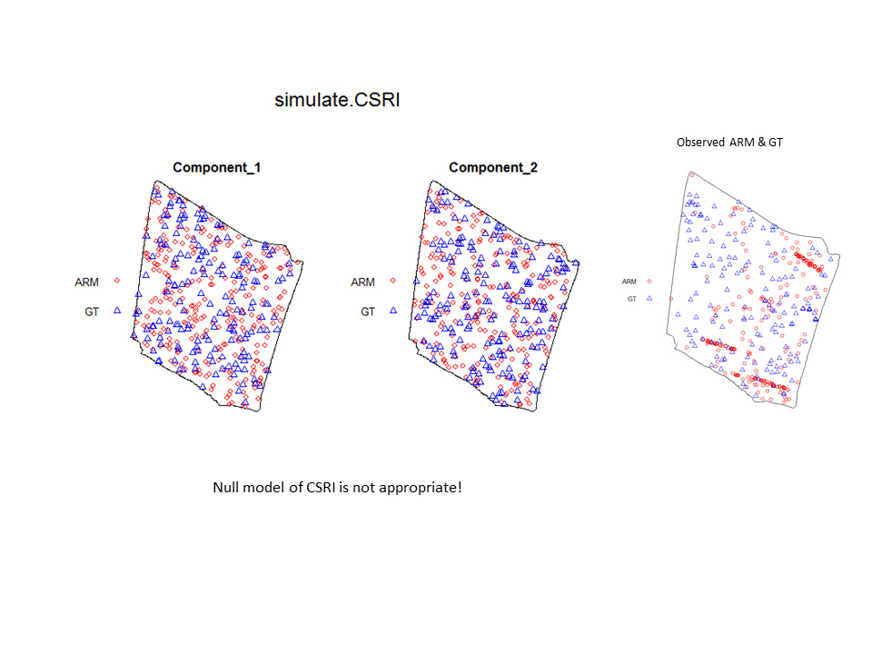
The Model and Monte Carlo approach works well when you can model the drivers of inhomogeneity (and given you fix the number of points in the simulations to match the observed pattern to account for the composite null hypothesis), but what happens when important covariates cannot be modeled? In such cases, the initial default is to use the x– and y-coordinates as predictors in a model, but this only works well if the inhomogeneity can be captured by a simple polynomial function and if you can rescale your coordinates in such a way to prevent numerical overflow. Another option is to use nonparametric kernel smoothing to create a covariate surface from which intensity can be estimated and simulated. From my own experience, I have found that this works well when the pattern of inhomogeneity is rather simple and there are not patches with extreme high intensity. For example, note how simulations based on the kernel smoothed intensity surface for armadillo burrows (with bandwidth selection based on maximum likelihood cross validation; a recommended method for inhomogeneous patterns) produces simulated point patterns that do not adequately reflect the observed pattern. The kernel tends to oversmooth the area around the dirt berms and simulated patterns based on this surface underestimate intensity within the berms and overestimate intensity around the margins of the berms.
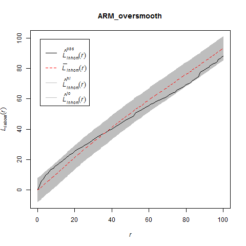
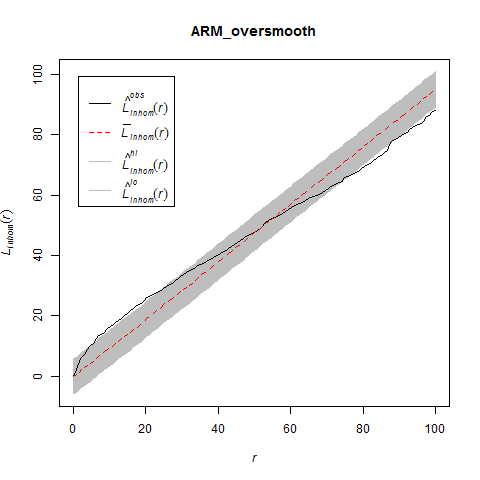
If you used this kernel smoothed surface to correct for inhomogeneity, you would expect it to under-correct the intensity at short distances between points on berms and over-correct intensity at longer distances between points in and around berms. Here are the L-functions (with significance envelopes) for the uncorrected pattern and for the pattern that has been corrected for inhomogeneity using the kernel-smoothed surface (above). For the uncorrected pattern, there is stong rejection of CSR in the direction of clustering (see ‘naive_Lest’). For the inhomogeneous L-function, it under-corrects at short distances between points and over-corrects at longer distances (presumably due to mis-estimation of the intensity in and around the berms).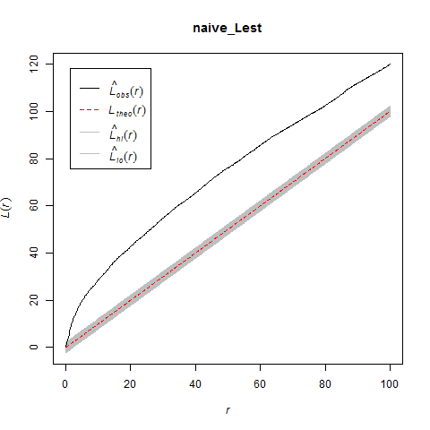
The problem is even more severe if you use the default bandwidth selection method (which results in even more extreme oversmoothing for this sort of pattern).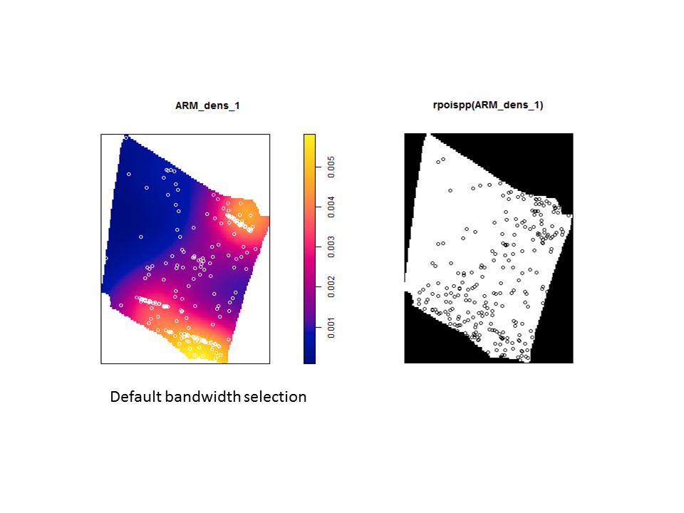
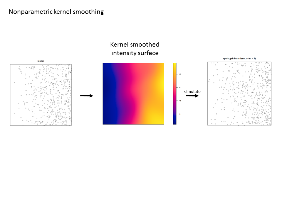
For simpler patterns (here a simple trend in intensity along the x-coordinate), kernel smoothing works pretty well and passes the “eyeball test” (i.e. the simulated pattern resembles the observed pattern).
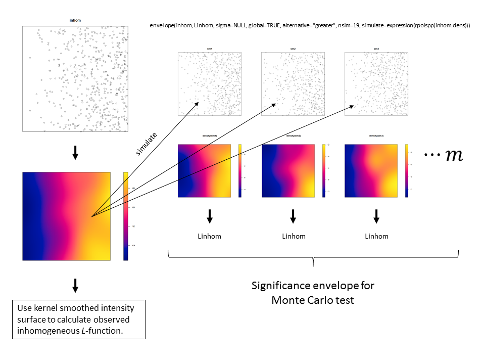
 For a univariate point pattern like this, the awesome developers of ‘spatstat’ have provided the code to use kernel smoothing to create a significance envelope for an inhomogeneous summary function (which can be found on the help page for the envelope() function). Here is an excerpt from the help file (using the Kinhom function as an example), followed by my own visual demonstration of the procedure (for Linhom ()).
 # Note that the principle of symmetry, essential to the validity of
 # simulation envelopes, requires that both the observed and
 # simulated patterns be subjected to the same method of intensity
 # estimation. In the following example it would be incorrect to set the
 # argument 'lambda=red.dens' in the envelope command, because this
 # would mean that the inhomogeneous K functions of the simulated
 # patterns would be computed using the intensity function estimated
 # from the original redwood data, violating the symmetry.  There is
 # still a concern about the fact that the simulations are generated
 # from a model that was fitted to the data; this is only a problem in
 # small datasets.

## Not run:
 red.dens <- density(redwood, sigma=bw.diggle)
 plot(envelope(redwood, Kinhom, sigma=bw.diggle,
         simulate=expression(rpoispp(red.dens))))
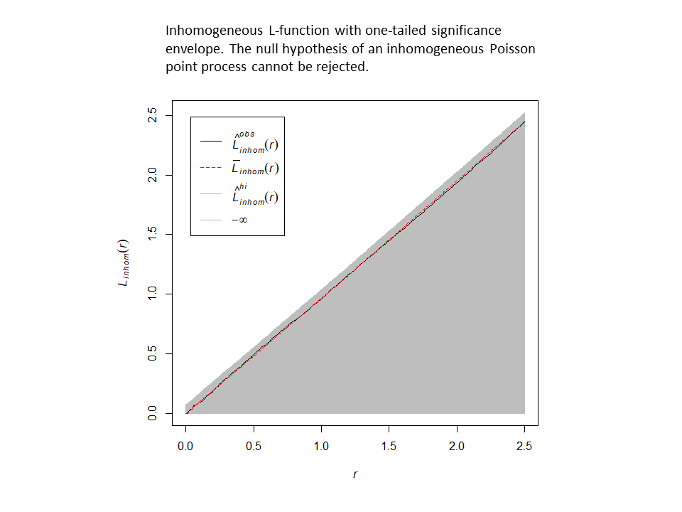
This procedure adequately corrects for the inhomogeneity. Here are the results for a one-tailed test (alternative = “greater”) with and without correction for inhomogeneity. Without correction, the null hypothesis is rejected in the direction of clustering…but, after correction, the null model of an inhomogeneous Poisson point-process cannot be rejected.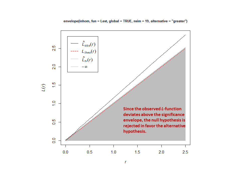
So what do you do if you are analyzing a bivariate pattern that exhibits inhomogeneity that cannot easily be modeled? We ran into this problem at one of our study sites (at the Lake Louise Field Station in Lowndes County, Georgia) where we know there is inhomogeneity associated with vegetative density, but for which no LiDAR data was available. The bivariate point pattern for armadillo (= ARM) and gopher tortoise (= GT) burrows looks like this (within a rectangular subregion of the plot):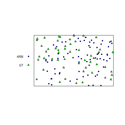
For the the bivariate pattern (shown above), one cannot reject the null hypothesis of CSRI using a two-sided simultaneous significance envelope (i.e., the observed L-function, represented by the black line, does not deviate outside of the (gray) significance envelope). However, there is some suggestion that the points of each type are bit more spaced out than expected (note that the summary function tends to deviate below the theoretical expectation, represented by the red-stippled line).
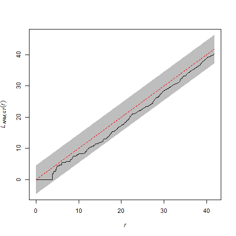
This is probably not a fluke because I know that the armadillo burrows are concentrated in some areas in the northeastern part of the study area window where there are thickets of hardwood saplings. I also know that there are more gopher tortoise burrows in the northwest corner of the study area window, where the canopy is more open and the understory is more herbaceous. Therefore, correction for inhomogeneity should probably be done, if possible.
Unfortunately, I ran into problems using the x– and y-coordinates as predictors (which were in UTMs); even when I rescaled the coordinates, I had persistent problems with numerical overflow. The last resort was to try to using kernel-smoothed intensity surfaces, which seemed to pass the simulation “eyeball test” for each species.
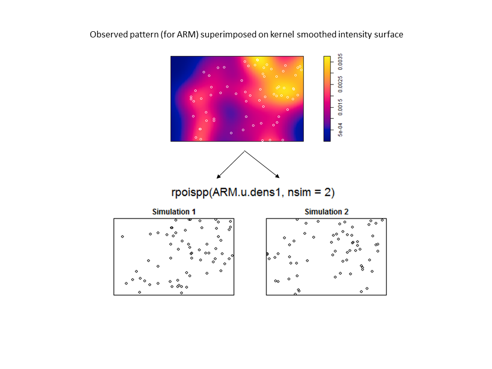
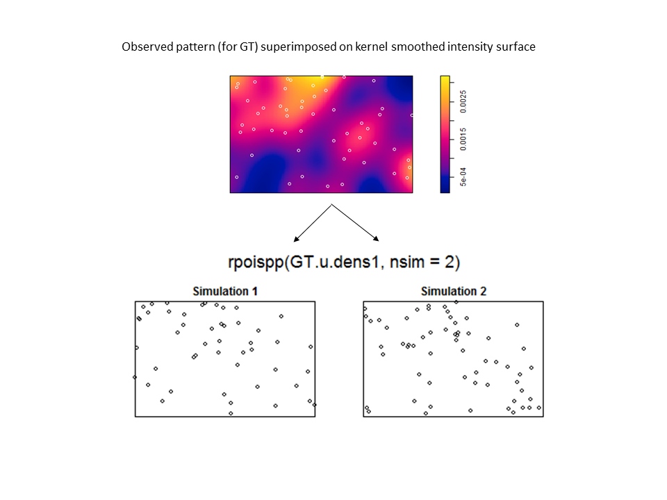 However, there are no examples in the help files (or in the book) if you want to use the kernel smoothed intensity surfaces for the purposes of correction (and envelope building) in a cross-type summary function. Nevertheless, by virtue of the flexibility of statistical programming (with existing functionality from ‘spatstat’), one can craft a solution in R. The trick is to write two custom functions to be used in the call to the envelope function. The first function (which I named smooth.LCI) is fed to the argument ‘simulate’. It takes the observed bivariate pattern, splits it into two patterns for each species, kernel smooths each pattern, simulates from each kernel smoothed surface, and then recombines them into a single bivariate pattern. The second function (calc.LCI) works on both the observed and simulated patterns. It takes the bivariate pattern, splits it, creates a new smoothed surface for each pattern, and then uses these surfaces to correct for inhomogeneity.
smooth.LCI <- function(X,…){
arm <- split(X)[[1]]
gt <- split(X)[[2]]
arm.dens <- density(arm)
gt.dens <- density(gt)
arm.sim <- rpoispp(arm.dens, fix.n=TRUE)
gt.sim <- rpoispp(gt.dens, fix.n=TRUE)
new <- superimpose(ARM=arm.sim, GT=gt.sim)return(new)
}calc.LCI <- function(Y,…){
arm2 <- split(Y)[[1]]
gt2 <- split(Y)[[2]]
arm.dens <- density(arm2, at=”points”)
gt.dens <- density(gt2, at=”points”)
Lcross.inhom(Y, “ARM”, “GT”, arm.dens, gt.dens)
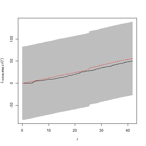
}plot(envelope(burrows2a, calc.LCI, simulate=smooth.LCI, nsim=39, global=TRUE))
After correction, there is still evidence of a wee-bit of repulsion between the different types of points, but it is less severe and well within the range of what might be observed for a bivariate Poisson point-process that is inhomogeneous.
Therefore even though this procedure is not described, it is possible. That’s the beauty of statistical programming: you are no longer bounded by the options in a menu. You can use existing functionality to create new functionality. You are freed from the GUI cave.